Two documents are available for this tutorial. One is a printable version of the text found beneath the video with full sized images, and the other is a "read-along" version that has thumbnails aligned with the script for the video.
This tutorial will walk you through the steps of processing the data from an X-ray diffraction experiment using HKL-2000. If you need to install HKL-2000, please see the instructions at the HKL Research website (http://www.hkl-xray.com/download-instructions-hkl-2000).
The data used in this and other HKL Research tutorials can be found at the Integrated Resource for Reproducibility in Macromolecular Crystallography at proteindiffraction.org. This tutorial will walk you through the process of indexing and scaling the dataset for 1WQ6 (doi:10.18430/M30592).
When you download the data from the IRRMC, the data will come packaged as a tar file that contains the diffraction images and the “site file” that is necessary to process the data. The site file (named def.site) contains information about the X-ray detector and other parameters that describe the experimental setup. The most important parameters are the type of detector and the position of the direct beam. The standard location for site file is /usr/local/hklint. Within the hklint directory, each experimental site is defined by directory with a descriptive name which contains a def.site file with details about the site.
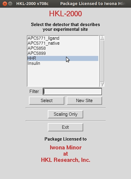
When you start HKL-2000, you are first presented with a list of experimental sites. For this tutorial, we will use the site called HHR, which corresponds to an ADSC-Q4 detector. Click on the HHR site to highlight it, and then click Select.
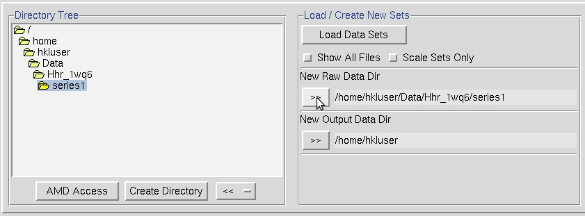
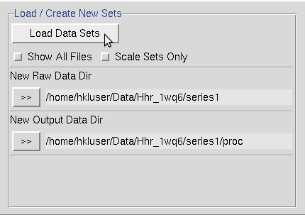
In order to tell HKL-2000 where to find the experimental data, use the Directory Tree on the left to navigate to and select the directory where the diffraction images are and click the double arrow button in the New Raw Data Dir field.
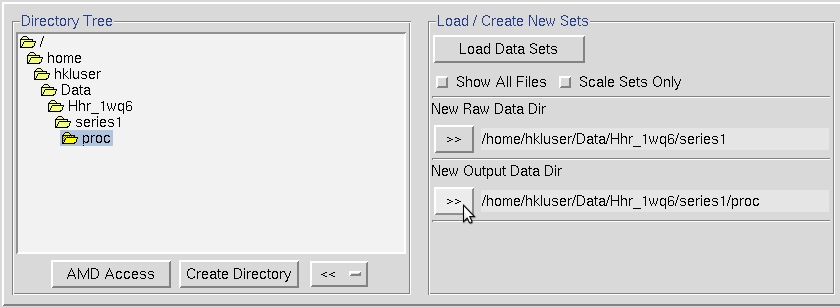
It is a good idea to create a new directory for the program output to keep the original images separate from the files that result from processing the image. To do so, will click the Create Directory button. A common practice is to create a subdirectory in the data directory called ‘proc.’ After creating a directory, select it and click the double arrow button in the New Output Data Dir field.
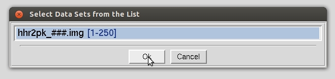
Select the images you want to process using the Load Data Sets button in the middle of the interface. This will open a dialog with images grouped by a file name pattern, followed by the range of images that fit the pattern. Here we see that there are 250 images that start with hrr2pk.
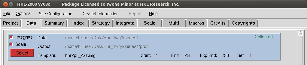
Each set of data will appear in a separate box in the data window. Here we only have one set, but other experiments may have more than one which may correspond to different wedges of data or different data collection parameters, such as distance, framewidth, wavelengths, etc. The parameters for each set can be viewed in the Summary tab at the top.
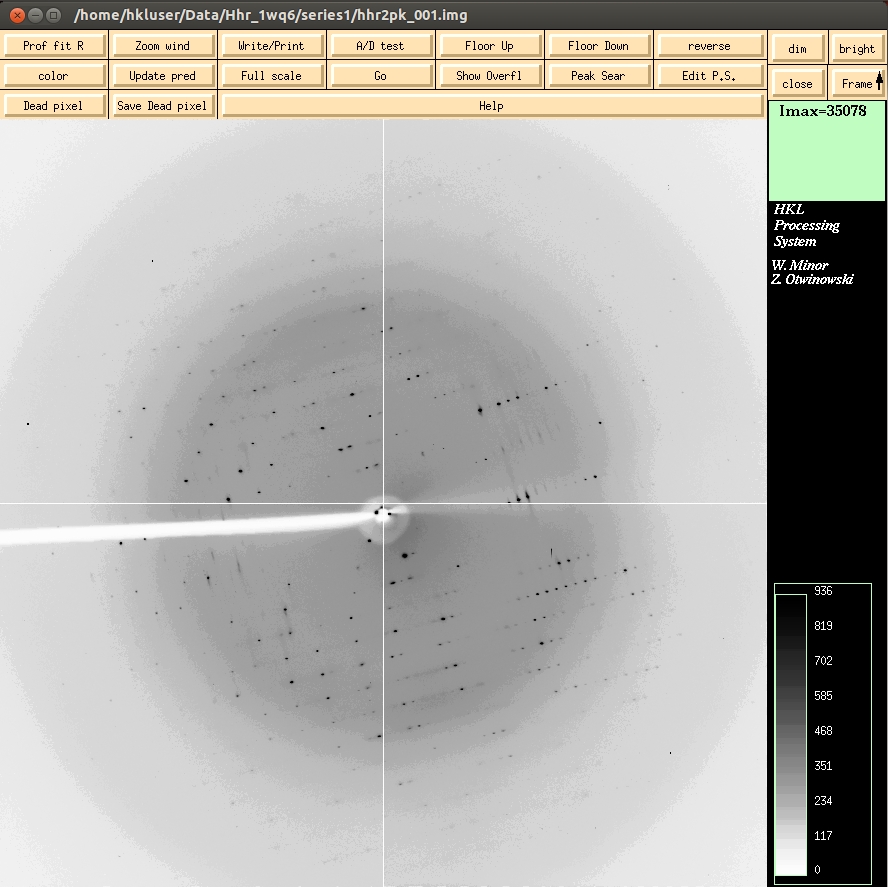
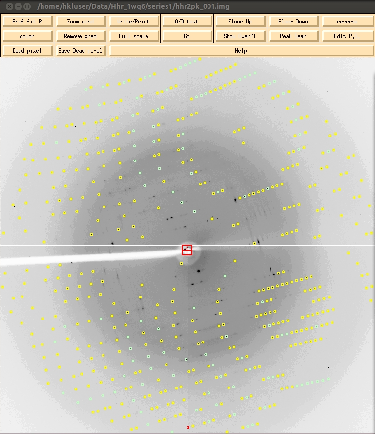
To see the first image of the dataset, click the Display button, which is under the Data tab. The bright and dim buttons in the upper right allow you to adjust the contrast for the images. The Frame button allows you to scroll through images. Middle clicking on the Frame button will display the next image in the direction of the arrow. Left click to change the direction of the arrow to down, right click to change the arrow to up. A Zoom window can be opened to get a better look at individual reflections. Middle clicking on the main image or zoom window will re-center the zoom window. Zoom in far enough and you can see the photon counts for each pixel.
The first step of indexing the data is to “peak search” the data. There are two ways to do this. The first is to select the Peak Search button at the top of the image display. This opens a dialog on the right that provides ways to alter the number of peaks selected. The Frame/Up button can be used to select peaks on more than one image, which can be useful in difficult cases. The Pick (Add) and Pick (Remove) buttons are very useful for weak data or if you need to select one crystal lattice from an image that clearly contains reflections from more than one crystal. Click OK when you are done. This saves the peaks to a file.
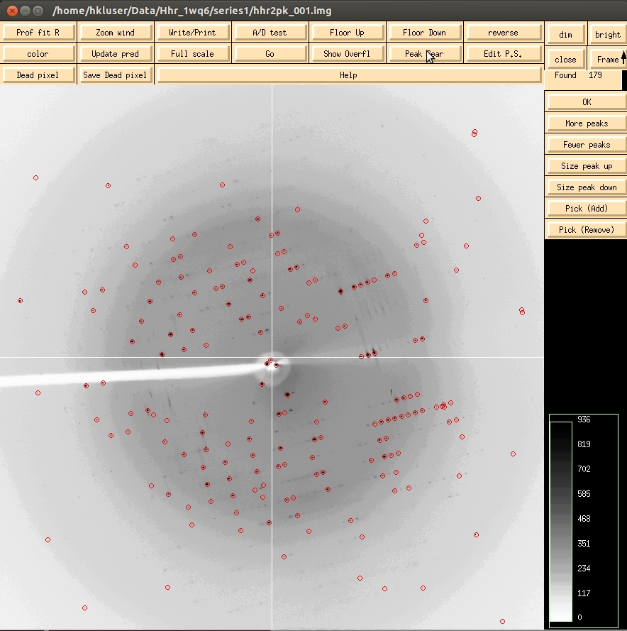
Because the default parameters for peak selection are usually sufficient, the alternate way perform a peak search is to switch to the Index tab and select Peak search. This will automatically select peaks from the first frame. It will also display the image if you have not previously done so.
The first step of processing the data is to index the reflections on the first image. This assigns Miller indices to each reflection. To start the process, switch to the Index tab.
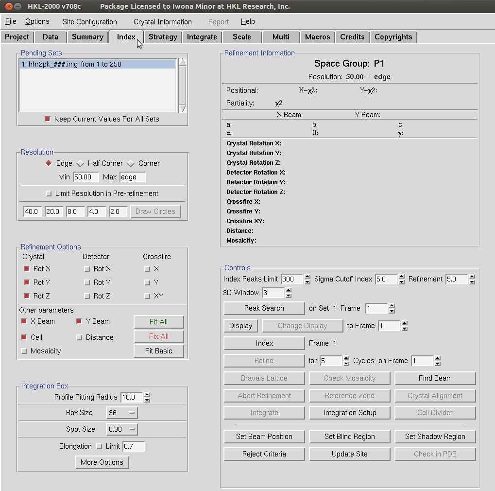
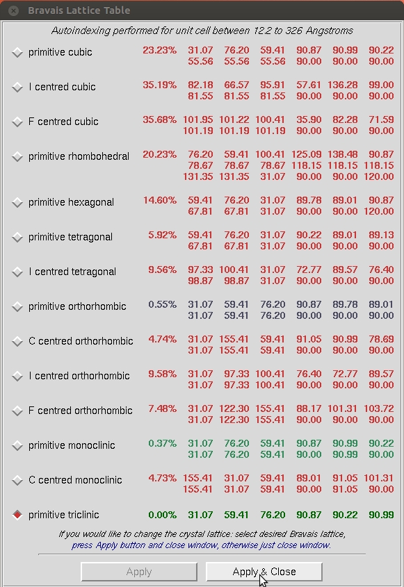
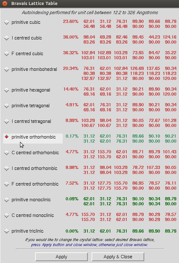
The Index button within the Controls box will try to auto-index the peaks using into all of the Bravais Lattices and presents a table with the Bravais Lattices types ordered from higher to lower symmetry. Each crystal class is presented with two unit cell values—the first is a primitive triclinic unit cell that fits the data and is closest to the a unit cell that compatible with that crystal class and then second row is the unit cell that would be necessary for that crystal class. For example, primitive tetragonal crystals have a= b and all angels = 90. Each crystal class is presented with a correlation coefficient that represents how well these two unit cells agree. HKL color codes the fit from dark green through navy to red. Sometimes you may select the crystal with the highest symmetry with a good correlation coefficient, but a better practice is to initially select the P1 unit cell and refine the unit cell before selecting the crystal class. To do this, Apply & Close this window while the primitive triclinic lattice is selected.
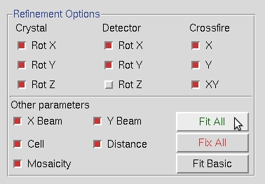
In order to get a better idea of which crystal class the crystal belongs to, you need to refine the primitive unit cell, the direct beam position (X Beam and Y Beam), and a few other parameters related to the crystal orientation (Crystal Rot X, Rot Y, and Rot Z). To refine these parameters, click the Refine button in the Controls Box.
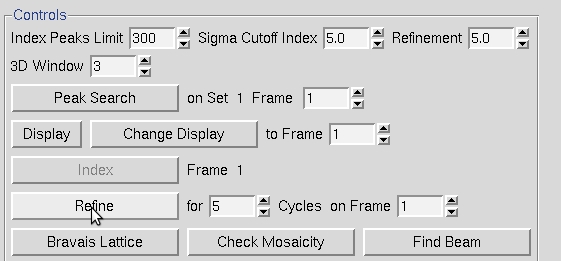
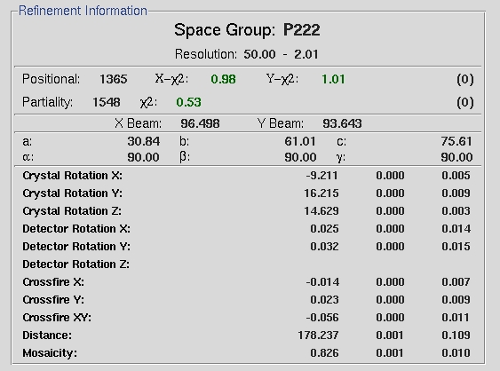
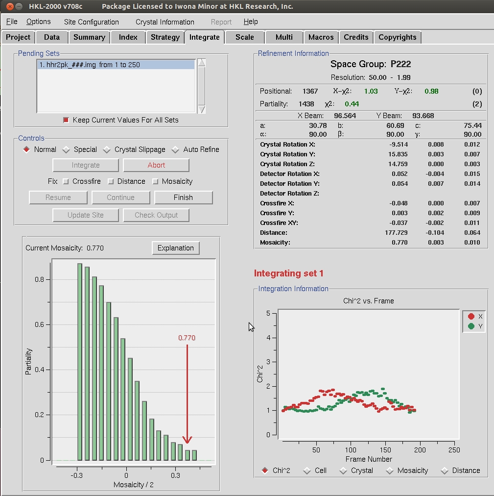
When the Refine button is clicked, the parameters selected in the Refinement Options box will be refined the number of times selected in the selector box next to the Refine button. The overall measurements of how well the selected crystal class fits the data are the Positional and Partiality Chi Square values. These are also color coded from dark to green to red from good to bad. The other refinement parameters that are refined are presented with their current value, how much they have changed during the refinement cycle, and the error associated with the value (from left to right). Click Refine several times and the values should become stable.
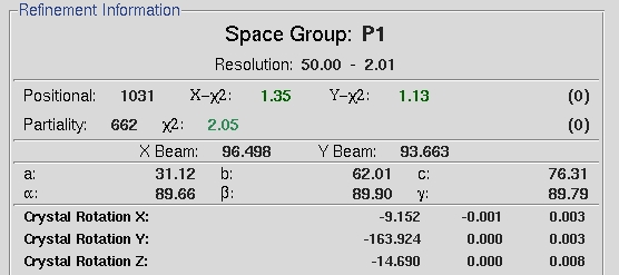
At this point the predicted reflections displayed on the image are color coded. Reflections that are recorded completely on this image will be green, whereas reflections that are split between more than one image will be yellow. These “partial” reflections will be combined during the scaling process. Reflections that are red have been rejected, perhaps because the background of the spot is not uniform, the selected spot size is too small for the reflection, or the reflection overlaps with another reflection. Keep an eye on the reflections during the refinement and integration process. The presence of too many rejected reflections is an indication that your indexing could be wrong, and will probably be accompanied by a spike in the chi square values. The presence of many reflections that are not predicted is an indication that the mosaicity is too low. It has not yet been refined in this image.
At this point, revisit the Bravais Lattice table and notice that the primitive orthorhombic class is the highest symmetry lattice type with a low correlation coefficient. Select this lattice and Apply & Close this window.
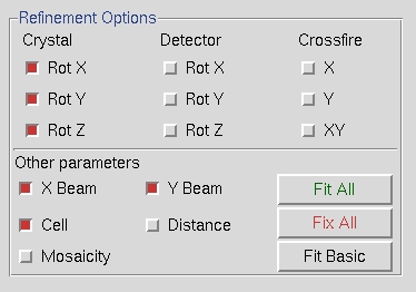
You can then add more parameters by selecting Fit All in the Refinement Options box. Click Refine until all the parameters become stable.
If the chi square values shoot up dramatically during refinement, you should abort the refinement and index the data again. The peak search data is saved in a file, so the peak search does not have to be performed again unless you want to change the peaks you are working with. This data set indexes easily, but that will not always be the case with every data set you collect. Some things that can help index more difficult data sets include:
- Increase the number of peaks that are used for the indexing
- Increase the sigma level used for indexing. Decrease the sigma level for extremely weak data.
- Change the high resolution limit until indexing works. Try 4 Å.
- Increase the number of frames used for indexing by picking peaks from several frames.
- Index the data on a different frame, perhaps 30 degrees from the first frame.
- Use Pick (Remove) during peak picking to remove reflections from a second lattice.
One other issue that you may run into with other data sets is that one of the Crystal Rotation parameters will be colored red. This is a minor issue that can be remedied by using the Reference Zone option to select one of the equivalent crystal orientations. Refine after selecting a different crystal orientation and the Crystal Rotation parameter should change to black.
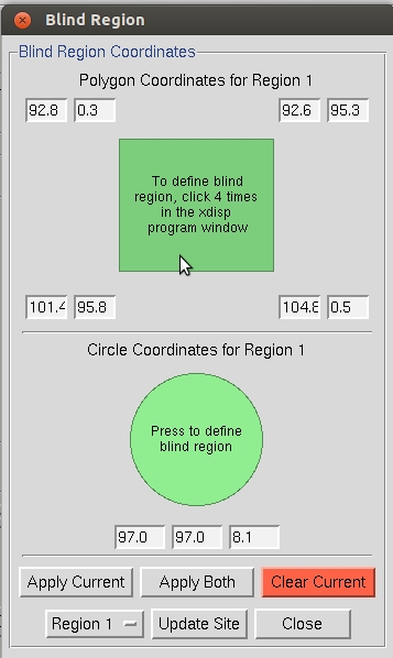
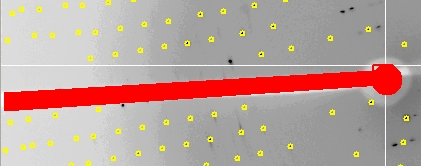
It is a good practice to mask the shadow of the beamstop to avoid including reflections that have been attenuated because they are partially obscured by the beamstop. This is especially important when using anomalous data during the structure determination process. Click Set Blind Region to see or edit the blind region. If the Blind Region dialog opens has values when you open it, then the blind region has already been set in the def.site file. If the values are missing or the position of the beamstop has changed, use the dialog to set a new mask. Two types of masks can be used, alone or together: a polygon determined by four corner points and a circle determined by a center point and a radius.
Once you are satisfied with the refined parameters and the blind region, use these parameters to integrate the whole dataset. This will index each individual frame and record the intensity and error associated with each peak. The process can be started with the Integrate button in the Index tab, which will automatically switch the display to the Integrate tab. Alternatively, use the Integrate button on the Integrate tab to start the process. HKL-2000 will then process each available image. The image will be displayed, peaks will be predicted, and the parameters will be refined for each image. The display will show a mosaicity histogram for the image being indexed and a cumulative graph on the right. The buttons at the bottom let you examine various parameters.
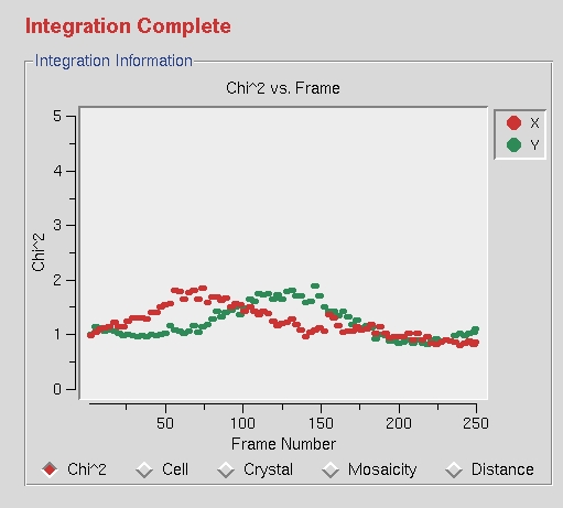
Once all the frames have been processed, the phrase “Integration Complete” will appear above the Integration Information window.
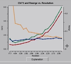
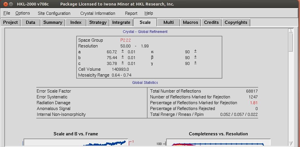
Once integration is complete, it is time to scale the data from the individual frames together. To do this, switch to the Scale tab and click the Scale button. This process normalizes the intensity of all of the frames, combines the data from the partial reflections, and merges symmetry related reflections. Scaling is an iterative process, so expect to have to use the Scale button numerous times. Each time scaling is complete, the Global Statistics at the top, as well as the various graphs that are presented. A number of diagnostic graphs are also presented, and can be access using the scroll bar on the right side of the top window. You can click on the Explanation button under each graph to see what each line represents.
A good approach to determine the spacegroup is to initially scale the data in the lowest symmetry spacegroup for the crystal class and then select use the Check Space Group button. This assumes that CCP4 is installed and HKL-2000 is configured to use it, and uses the CCP4 program POINTLESS.
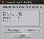
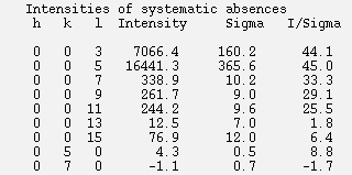
However, to show the process using HKL-2000 alone, this tutorial assumes that you do not have CCP4 installed, and demonstrates the process of examining the space group manually. Screw axes will result in some reflections that are systematically absent, and these reflections are listed in the log file to make it easy to evaluate if these reflections are present or absent. Primitive orthorhombic crystals can have three screw axes, so selecting P212121 and scaling the data will allow all of the possible screw axes to be evaluated. Use the drop down menu next to Space Group drop down menu to select Primitive Orthorhombic then select P212121. The reflection that should be systematically absent for the selected space group are displayed at the end of the scaling log file, so select Show Log File and scroll to the end to see the reflections listed along with their average intensity, error and I/sigma values.
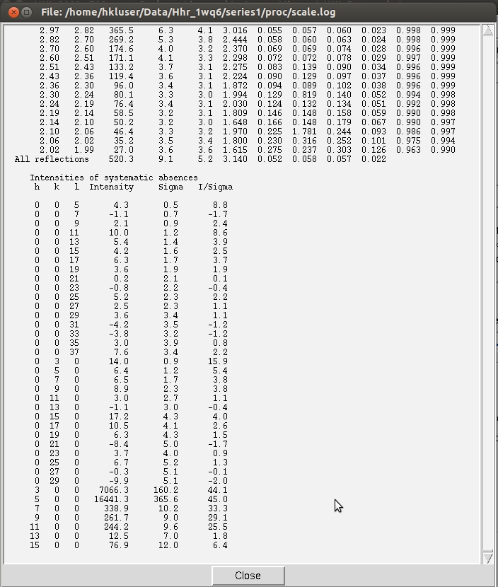
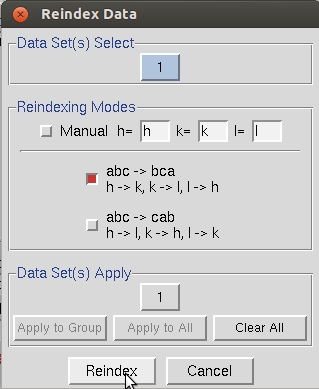
As can be seen in this case, the reflections hodd 0 0 are present, although the reflections 0 kodd 0 and 0 0 lodd are indeed absent. This indicates that this crystal has two screw axes, along b and c. Note that this is consistent with the CCP4 output shown above. However, the crystallographic convention for a primitive orthorhombic space group with two screw axes is to have the two screw axes along a and b axes. To rectify this, we use the Reindex option from the Controls box.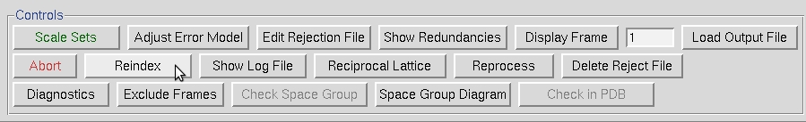
Select the option that converts abc into bca and select Reindex.
If the data is then rescaled in P212121, the list of systematic absences at the end of the log file will indicate that the screw axis is now along the c axis, consistent with the crystallographic convention.
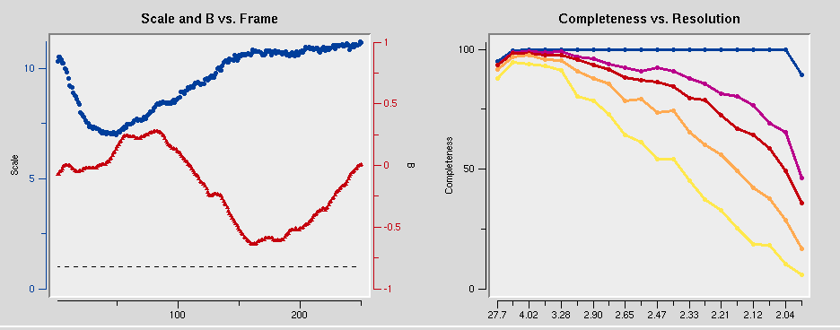
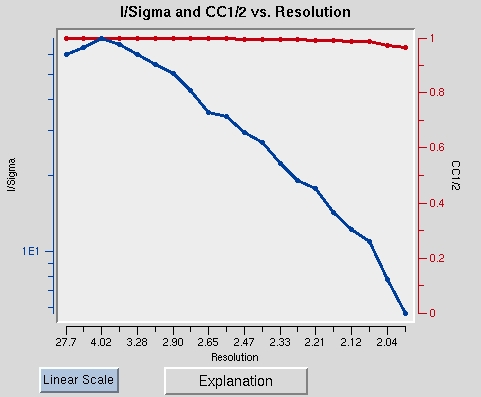
Scaling the data is an iterative process. The first passes can be used to determine resolution limits and the overall Error Scale Factor. To set the resolution limit, look at the graph of I/sigma vs Resolution. This also has a graph of the CC1/2, which is another parameter that some people use for setting the resolution limit. If your data is weaker than two sigma, a line will appear on the graph suggesting a resolution to truncate your data. This is strong data, so we will use all of it. Set the upper and lower limits of the data based on the strength of diffraction and the size of the beam stop.
In the absence of an anomalous signal, the Error Scale Factor can be increased if too many reflections are being rejected, but in this example, we know that we intend to use the anomalous signal from the data to solve the structure, so we will select the Anomalous button and then Scale again. This will ensure that the Friedel pairs are not merge, meaning that the hkl reflections are not merged with the –h-k-l reflections. The anomalous signal is incredibly strong in this data set, and scaling with the Anomalous option dramatically decreases the Number of reflections Marked for Rejection.
Once the some of the key parameters of the scaling process have been determined, select Use rejections on next run to exclude these reflections from the scaling process. Scale the data a few times until the number of reflections marked for rejection stabilized and the global statistics are also stable.
At this point, you can get a feel for whether or not the structure can be determined using the anomalous signal. In the graph of Chi square vs resolution, the blue line represents the chi square values when Friedel pairs are kept separate, and the orange line represents the chi square values if when the Friedel pairs are merged. The fact that the chi squares are higher when they are merged indicates that there is a measurable difference between the Friedel paris, which indicates an anomalous signal. This example has one of the strongest anomalous signals you may ever see. You can usually solve the structure if there is even a modest difference between these two lines at lower resolutions, and it will certainly work in this case.